How to Setup Anomaly Analysis
This document describes a recommended approach for configuring automated anomaly analysis on enterprise data. The guidance aims to produce effective, comprehensive analyses that can be exposed as role-based views. The following chapters present a practical, step-by-step method.
How to Start
AnomalyGuard is designed so a typical data engineer or data/business analyst can configure it without programming or complex setup.
The infrastructure team should first install the application in the company environment and then, together with data engineers, define connectors to the source datasets.
One-person setup
A single experienced analyst can perform the configuration described in this chapter. It is important that this person understands the data and the company's business context in order to define which changes matter for which roles (CEO, CFO, regional/product managers, data quality team, etc.). Different roles will care about different types of anomalies and dimensions.
Before starting, choose the datasets you will analyze.
Choose Data
When rolling out AnomalyGuard, start with datasets that are important across the company and whose results affect many teams. Typical examples are core datasets such as product sales over time, with relevant categorical dimensions. The example below shows a revenue datamart for a hotel chain.

This is a high-value dataset: its analysis influences business operations and many employees. Anomaly detection on such data can deliver wide-ranging value.
Select the dataset and the relevant dimensions you want to analyze. From this dataset you will create one or more Data Views.
Create Data View
The technical steps for creating and managing Data Views are described in Data Views. Here we focus on the methodological decisions.
When you have source data available, decide whether to create a single Data View or multiple Data Views for the dataset.
This decision depends primarily on the complexity of your data. The sample dataset above contains multiple categorical dimensions; analysis will evaluate combinations of these dimensions (e.g., a selected hotel and payment method). The number of combinations can quickly grow to tens of thousands.
If you run analysis weekly (for example, during weekend processing) a large number of combinations may be acceptable. For daily analysis with a requirement to produce results shortly after the warehouse load, more than ~20,000 combinations may become computationally expensive.
In such cases split the dataset into multiple Data Views — for example, one Data View for revenue by country/district/hotel and another for revenue by business source/market/payment method. Splitting reduces the number of combinations per view while still allowing detailed monitoring across all categories. Also note that analyzing at the lowest-combination level can produce mostly "data noise" where there are very few observations per combination.
Scaling compute
If you need fine-grained analysis and fast processing, you can scale compute resources (for example, increase the number of worker nodes in Kubernetes) via a Helm chart update or redeployment. The application database is separated from the application so deployments can be scaled without impacting the DB.
Once you know which subset of the data each Data View should monitor, define the Data View (load queries, categories, and metadata) as described in Data Views. Next, decide which variables to analyze.
Select Variables
For each Data View you can analyze one or more of the following variables: - Count - Value - Avg
Data Views are flexible across dataset types:
- Count represents discrete counts (e.g., items sold, served customers, inventory counts). This is an integer field.
- Value represents a numeric measure (e.g., revenue, price, metric readings such as temperature or flow, or financial values).
- Avg is computed as Value / Count and is not required in input data.
If you have only one observable variable in the input, set the other variable as a constant in the load query (for example SELECT 1 AS "Count") so you can later enable analysis on the second variable if needed.
When data, categories, and variables are defined, continue to the analysis setup.
Setup Analysis
Analysis configuration is performed in a few steps and tabs. Conceptually the setup consists of three parts: - Scan properties (how to pre-process input data before detection) - Detection functions (which detectors to run and their parameters) - Load settings (how and when to load and run analysis)

Setup Scan Properties
After the Load Query returns data in the expected format, define the scan properties. First, select the variables to analyze (see previous section). Then configure three important parameters: Fill Gap Method, Scan In Last N Days, and Ignore Last N Days.
Input data may contain gaps: some days may be missing for certain category combinations. This can occur for two reasons: a temporary technical outage (fixed on the next load) or genuinely no data for a period.
- For state variables (e.g., temperature), missing values typically indicate measurement outages — the value is not zero and should be filled with the last/next known observation or interpolated.
- For sum variables (e.g., daily sales), missing values usually mean no activity — the correct fill is zero.
Use Fill Gap Method to tell AnomalyGuard how to treat missing values. Options: - Zero — fill missing values with zero (typical for sums) - Previous — carry the last known value forward (useful for state measurements) - Linear Interpolation — interpolate between surrounding values
Scan In Last N Days limits how far back the analysis looks. This is useful if historical events (e.g., the COVID period) introduced anomalies you do not want included, or to speed up analysis by using a smaller date range. Set to 0 to use all available data.
Ignore Last N Days helps with late-arriving facts (data that arrives progressively). If recent days are incomplete, they may produce false anomalies. Setting Ignore Last N Days to 3 will exclude the most recent three days from analysis. Set to 0 to include all days.
Choosing Detection Functions
With variables and scan properties configured, define the detection functions (detectors) to use. Select detectors that match the use cases and the types of changes stakeholders care about.
Sometimes a single detector is sufficient; other times you may combine multiple detectors or multiple instances of the same detector with different parameters. Detectors are entered as simple function calls in a textbox and separated by semicolons. The text editor enables quick edits and rapid iteration. Example configuration:
Spike(0.35, 1024, 99.0, null, null, null)
Gap(1, 0, null, null, null)
MoM(70.0, above, null, null, null)
MoM(50.0, below, null, null, null)
Mpy(20.0, above, null, null, null)
Mpy(20.0, below, null, null, null)
WoW(50.0, above, null, null, null)
WoW(50.0, below, null, null, null)
Wpy(50.0, above, null, null, null)
Wpy(50.0, below, null, null, null)
Qt(0.1, below, null, null, null)
Qt(0.95, above, null, null, null)
DynamicThreshold(60, 3.0, None, null, null, null)
ClusterWindows(17, 1, 2, null, null, null)
All detectors share the same general structure:
function-name(function-parameters, common-parameters)
Common parameters (applied across detectors) are maxGapAmount, minValue, and minCount. These help exclude category combinations with insufficient data. If a parameter is NULL, that filter is not applied and the combination remains eligible for analysis. When set, the filters use metrics computed from the selected data (for example, percentage of missing days or long-term average of Value/Count).
Use these filters for two common cases: 1. Exclude combinations with too little data (e.g., a single SKU in one store with very few transactions). 2. Apply different thresholds for identifying anomalies in small vs. large categories. For example, a month-over-month drop of 200% might be a meaningful anomaly for small items, while for large categories you may want to flag drops of 50%.
Example: run a broad detector across all combinations and a stricter detector for large categories:
MoM(200, below, null, null, null)
MoM(50, below, null, 50000, null)
The first line flags relative changes across all combinations. The second line flags more moderate drops but only for combinations with average daily sales above 50,000 (using minValue or similar common parameter).
Tuning over time
Detection configuration can change over time. Each run overwrites previous results. Changes may be necessary because the data characteristics change (for example, corrected loads) or the nature of anomalies evolves (a short spike may later reveal a trend change).
Load definition
After detectors are defined, configure load parameters.
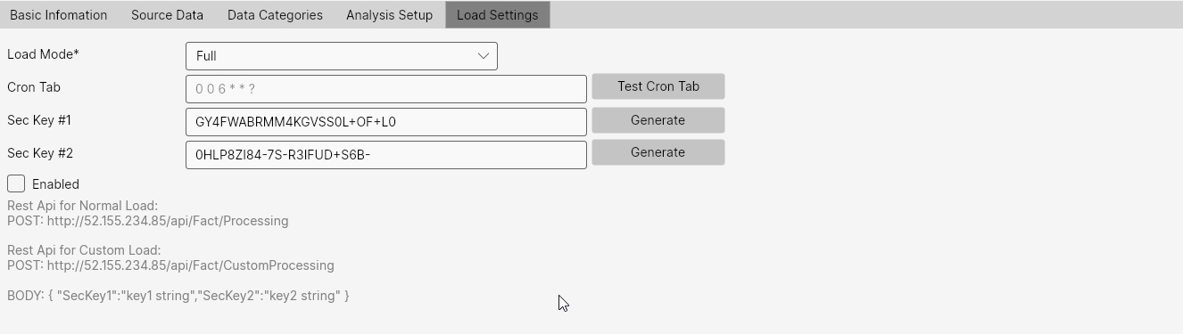
The Load Mode parameter determines whether the system performs a full reload or an incremental update. In Incremental mode, only new or updated rows are applied. In Full mode, existing data is deleted and reloaded. Incremental mode is recommended only when daily full loads would exceed ~10 million rows; otherwise Full mode is simpler and safer if source systems can handle it.
Next, configure how analyses are triggered. You can schedule automatic runs using Cron Tab, or enable external triggers by defining security keys for POST requests (useful to run analysis after an external ETL completes). See Data View properties in Data Views for details.
Detection Algorithms
The following section lists the detection functions available in AnomalyGuard. New versions may add or adjust detectors — contact support if you need an additional algorithm.
These detectors allow you to build relatively complex automated analyses that produce actionable outputs for different roles across the organization.
CW
The ClusterWindows (CW) function detects anomalies in data by identifying points that significantly deviate from the rest of the cluster. Data is divided into windows of size windowSizeDays, and clustering is applied within each window based on eps and minPoints, which define the density and size of clusters. Points that do not fit the cluster or are substantially different from others are marked as anomalies.

Command:
CW(windowSizeDays, eps, minPoints, maxGapAmount, minValue, minCount)
Parameters:
windowSizeDays- Required. The window size in days for clustering (default value is 30)eps- Required. The epsilon value for clustering (default value is 1)minPoints- Required. The minimum number of points for clustering (default value is 2)maxGapAmount– Maximum allowed proportion of missing data before analysis is skipped (default value is 5%).minValue– Optional minimum value threshold for anomalies (default value is null).minCount– Optional minimum number of points required for detection (default value is null).
Example:
CW(30, 1, 2, null, null, null);
CW(30, 1, 2, 5, null, 10);
CW();
DOD
The DoD function detects anomalies by comparing values between consecutive days. It flags points where the percentual change exceeds the specified percentualChange in the chosen mode ('above' or 'below'), highlighting sudden increases or decreases from one day to the next.
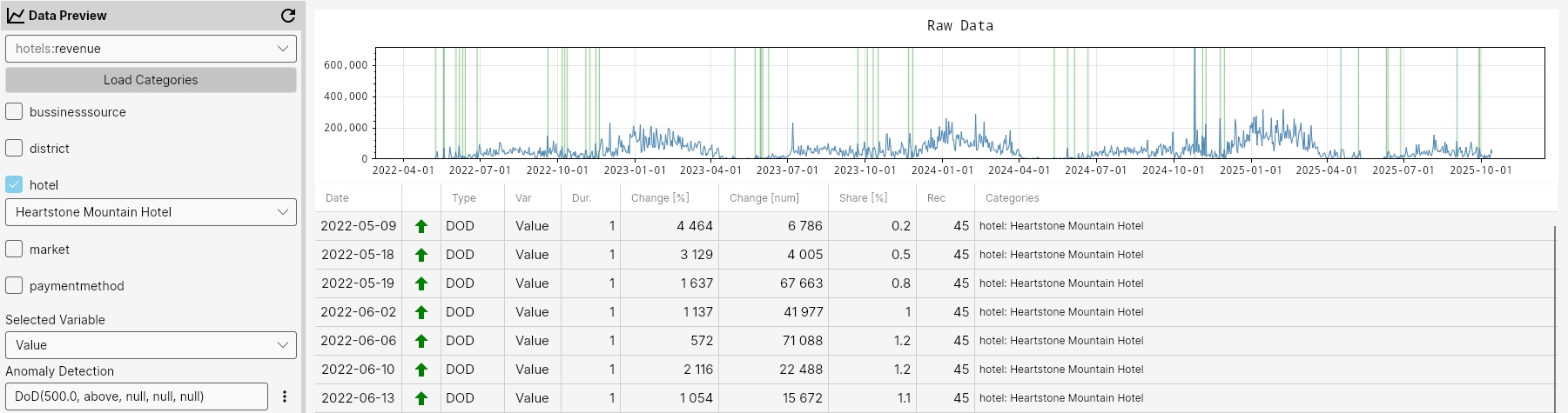
Command
Dod(percentualChange, mode, maxGapAmount, minValue, minCount)
Parameters
percentualChange- Required. The percentual change value for anomaly detection (default value is 50.0)mode- Required. The mode value for anomaly detection - 'above' or 'below' (default value is 'above')maxGapAmount– Maximum allowed proportion of missing data before analysis is skipped (default value is 5%).minValue– Optional minimum value threshold for anomalies (default value is null).minCount– Optional minimum number of points required for detection (default value is null).
Example
Dod(50.0, above, null, null, null);
Dod(50.0, above, 5, null, 10);
Dod();
DT
The DynamicThreshold (DT) function detects anomalies by identifying points that significantly deviate from a long-term dynamic threshold. It uses historical data spanning historyDays and applies a sensitivity factor to determine how much a point must deviate to be considered an anomaly. The function also accounts for seasonal patterns specified by seasonalityType, such as 'None', 'Weekly', 'Monthly', or 'Annual'. Points that exceed the dynamically calculated threshold based on these settings are marked as anomalies.

Command
DT(historyDays,sensitivity, seasonalityType, maxGapAmount, minValue, minCount)
Parameters
historyDays- Required. The history days for anomaly detection (default value is 60)sensitivity- Required. The sensitivity value for anomaly detection (default value is 3.0)seasonalityType- Required. The seasonality type for anomaly detection - 'None', 'Weekly', 'Monthly', 'Annual' (default value is 'None')maxGapAmount– Maximum allowed proportion of missing data before analysis is skipped (default value is 5%).minValue– Optional minimum value threshold for anomalies (default value is null).minCount– Optional minimum number of points required for detection (default value is null).
Example
DT(60, 3.0, None, null, null, null);
DT(60, 3.0, None, 5, null, 10);
DT();
Gap
The Gap function detects anomalies by identifying missing values in the data that stand out from the rest of the series. It can be configured to flag only gaps longer than longerThan days or shorter than shorterThan days, allowing precise detection of unusually long or short periods of missing data. Points that meet these criteria are marked as anomalies.
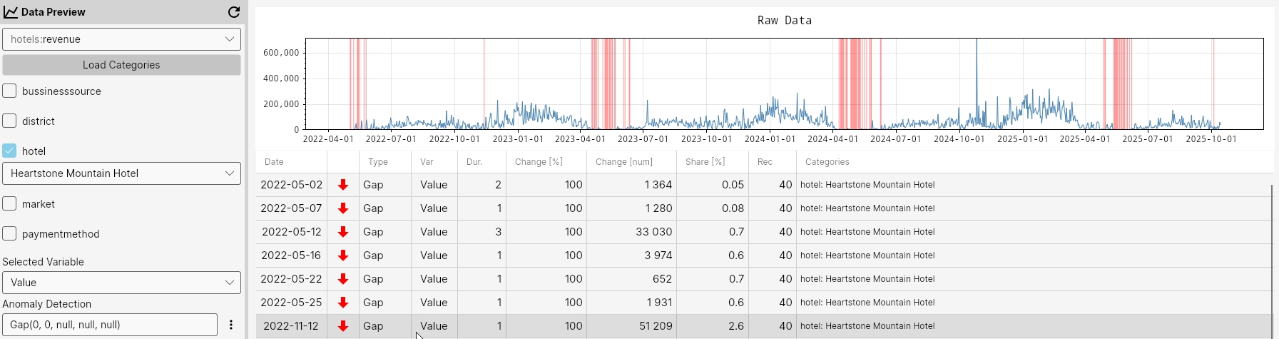
Command
Gap(longerThan, shorterThan, maxGapAmount, minValue, minCount)
Parameters
longerThan- Optional. Minimum length of gap (default value is 0).shorterThan-Optional. Maximum length of gap (default value is 0).maxGapAmount– Maximum allowed proportion of missing data before analysis is skipped (default value is 5%).minValue– Optional minimum value threshold for anomalies (default value is null).minCount– Optional minimum number of points required for detection (default value is null).
Example
Gap(0, 0, null, null, null);
Gap(0, 0, 5, null, 10);
Gap();
ChangePoint
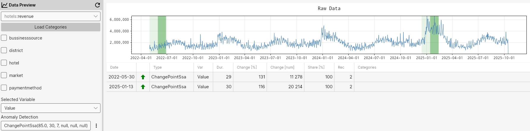
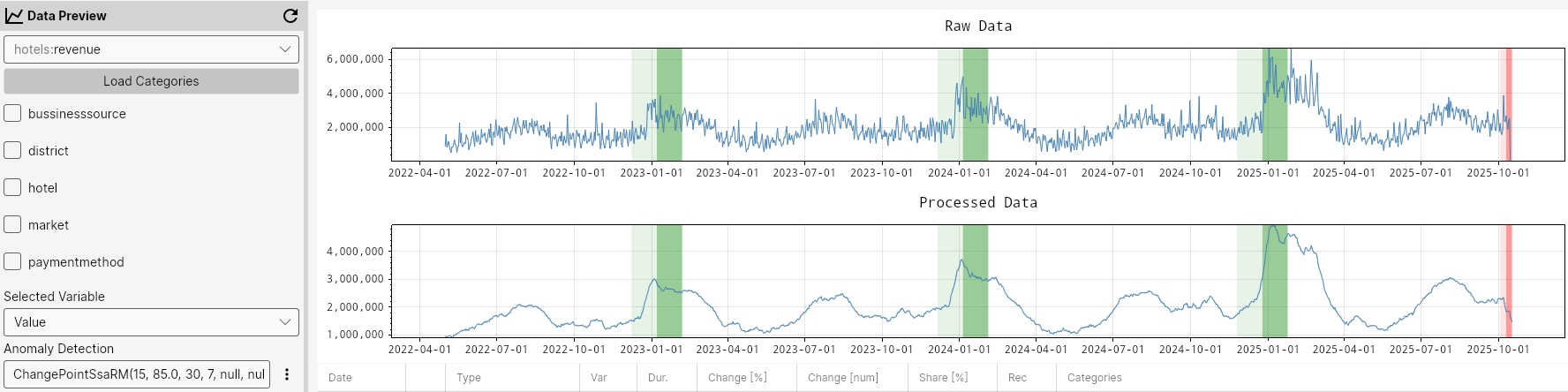
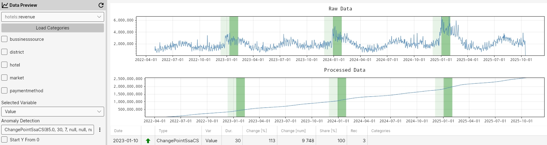
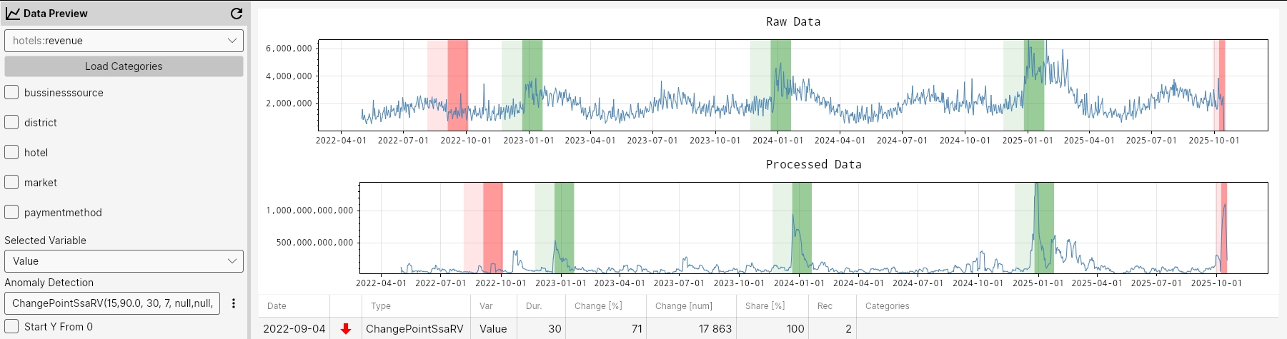
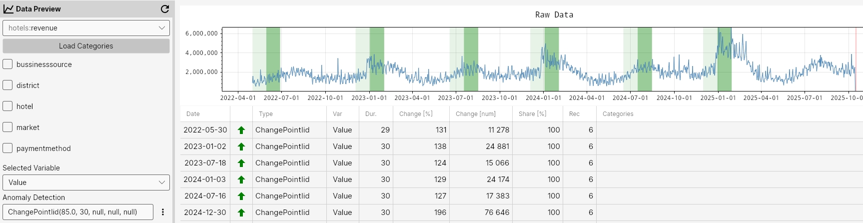
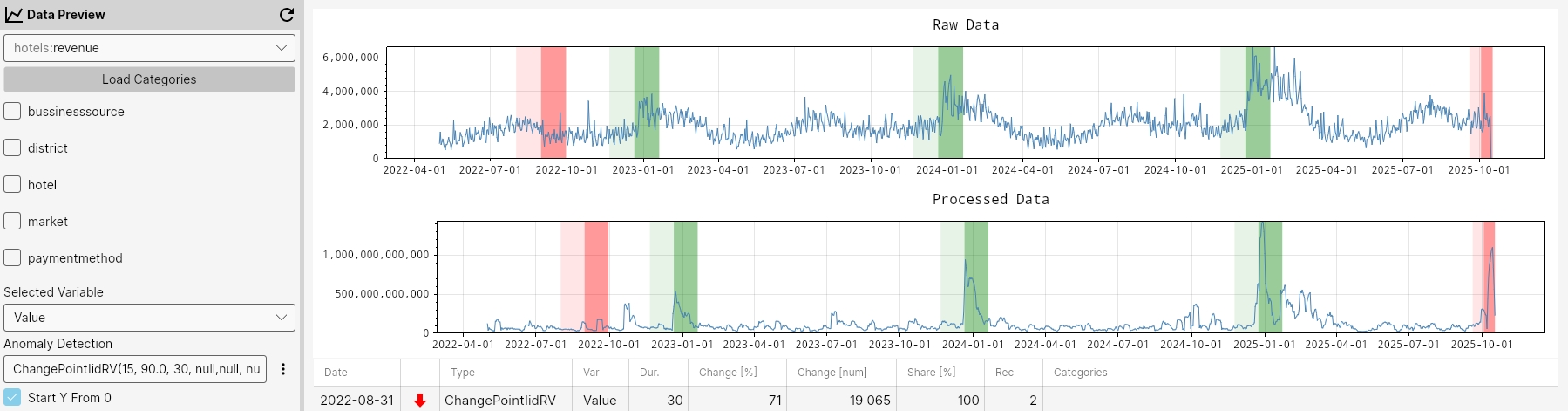
These functions detect structural changes or anomalies in time series data using two core algorithms: ChangePointSSA and ChangePointIID. They can be applied to different transformations of the data to capture changes at multiple levels.
Algorithms Overview
- ChangePointSSA: Suitable for data with trend and seasonality. Detects change points after adjusting for seasonality and trends.
- ChangePointIID: Assumes data is independent and identically distributed. Detects abrupt changes in mean, variance, or distribution. Suitable for stationary data.
Functions and Data Transformations
| Data Type | SSA Functions | IID Functions | Description |
|---|---|---|---|
| Raw Data | ChangePointSSA(confidence, changeHistoryLength, seasonalityWindowSize, maxGapAmount, minValue, minCount) |
ChangePointIID(confidence, changeHistoryLength, maxGapAmount, minValue, minCount) |
Detects structural changes in the original series. SSA accounts for trend/seasonality; IID assumes stationarity. |
| Rolling Mean | ChangePointSSARM(windowLength, confidence, changeHistoryLength, seasonalityWindowSize, maxGapAmount, minValue, minCount) |
ChangePointIIDRM(windowLength, confidence, changeHistoryLength, maxGapAmount, minValue, minCount) |
Detects persistent shifts in rolling mean values. SSA adjusts for trend/seasonality; IID assumes assumes stationarity. |
| Cumulative Sum | ChangePointSSACS(confidence, changeHistoryLength, seasonalityWindowSize, maxGapAmount, minValue, minCount) |
ChangePointIIDCS(confidence, changeHistoryLength, maxGapAmount, minValue, minCount) |
Detects changes in cumulative sums. SSA adjusts for trend/seasonality; IID assumes assumes stationarity. |
| Rolling Variance | ChangePointSSARV(windowLength, confidence, changeHistoryLength, seasonalityWindowSize, maxGapAmount, minValue, minCount) |
ChangePointIIDRV(windowLength, confidence, changeHistoryLength, maxGapAmount, minValue, minCount) |
Detects changes in rolling variance. SSA adjusts for trend/seasonality; IID assumes assumes stationarity. |
Common Parameters
confidence– Confidence level for change detection (e.g., 95%).windowLength– Size of rolling window (for RM and RV variants).changeHistoryLength– Number of past points to consider for detecting changes.seasonalityWindowSize– Size of the seasonal window for SSA-based functions.maxGapAmount– Maximum allowed proportion of missing data before analysis is skipped (default value is 5%).minValue– Optional minimum value threshold for anomalies (default value is null).minCount– Optional minimum number of points required for detection (default value is null).
Notes
- Use SSA functions for series with trend or seasonality.
- Use IID functions for stationary series or when trend/seasonality is not significant.
- Choose between raw, rolling mean, cumulative sum, or rolling variance depending on the type of shift you want to detect (level, trend, cumulative, volatility).
Examples
ChangePointSsa(95.0, 30, 7, null, null, null);
ChangePointSsaRM(15, 95.0, 30, 7, null, null, null);
ChangePointSsaCS(95.0, 30, 7, null, null, null);
ChangePointSsaRV(15, 95.0, 30, 7, null,null, null);
ChangePointIid(95.0, 30, null, null, null);
ChangePointIidRM(15, 95.0, 30, null, null, null);
ChangePointIidCS(95.0, 30, null, null, null);
ChangePointIidRV(15, 95.0, 30, null,null, null);
Screenshots
ChangePointSsa
ChangePointSsaRM
ChangePointSsaCS
ChangePointSsaRV
ChangePointIid
ChangePointIidRM

ChangePointIidCS
ChangePointIidRV
MOM
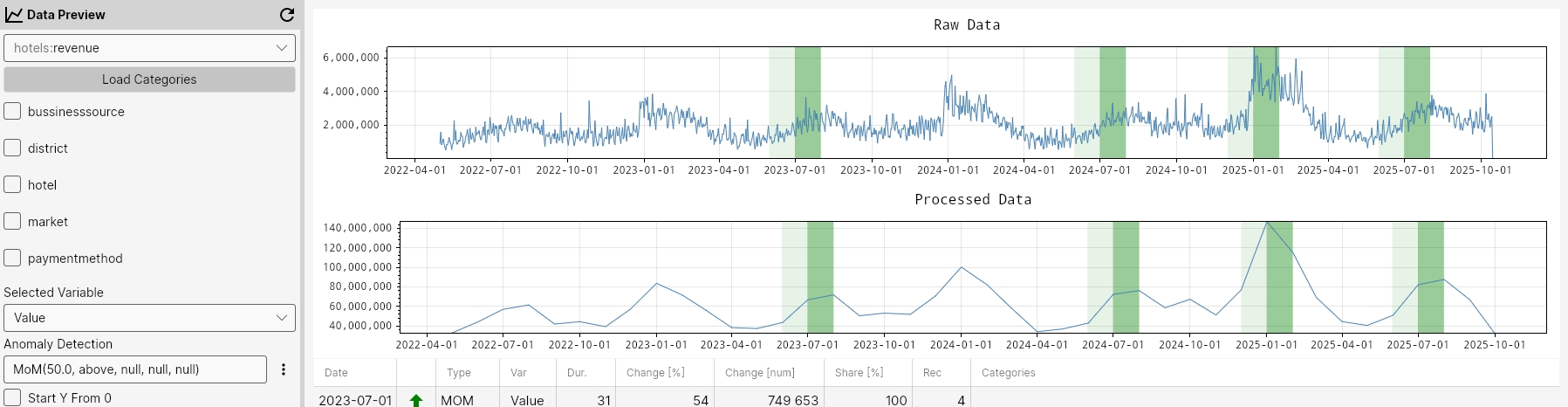
The MoM function detects anomalies by comparing values between consecutive months. It flags points where the percentual change exceeds the specified percentualChange in the chosen mode ('above' or 'below'), highlighting sudden increases or decreases from one month to the next.
Command
Mom(percentualChange, mode, maxGapAmount, minValue, minCount)
Parameters
percentualChange- Required. The percentual change value for anomaly detection (default value is 50.0)mode- Required. The mode value for anomaly detection - 'above' or 'below' (default value is 'above')maxGapAmount– Maximum allowed proportion of missing data before analysis is skipped (default value is 5%).minValue– Optional minimum value threshold for anomalies (default value is null).minCount– Optional minimum number of points required for detection (default value is null).
Example
MoM(50.0, above, null, null, null);
MoM(50.0, above, 5, null, 10);
MoM();
MPY
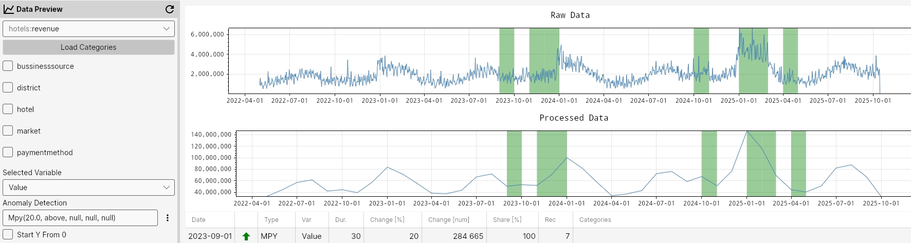
The MPY function detects anomalies by comparing values of a given month to the same month in the previous year. It flags points where the percentual change exceeds the specified percentualChange in the chosen mode ('above' or 'below'), highlighting significant year-over-year deviations.
Command
Mpy(percentualChange, mode, maxGapAmount, minValue, minCount)
Parameters
percentualChange- Required. The percentual change value for anomaly detection (default value is 50.0)mode- Required. The mode value for anomaly detection - 'above' or 'below' (default value is 'above')maxGapAmount– Maximum allowed proportion of missing data before analysis is skipped (default value is 5%).minValue– Optional minimum value threshold for anomalies (default value is null).minCount– Optional minimum number of points required for detection (default value is null).
Example
MPY(50.0, above, null, null, null);
MPY(50.0, above, 5, null, 10);
MPY();
QOQ
The QoQ function detects anomalies by comparing values between consecutive quarters. It flags points where the percentual change exceeds the specified percentualChange in the chosen mode ('above' or 'below'), highlighting significant shifts from one quarter to the next.

Command
QoQ(percentualChange, mode, maxGapAmount, minValue, minCount)
Parameters
percentualChange- Required. The percentual change value for anomaly detection (default value is 50.0)mode- Required. The mode value for anomaly detection - 'above' or 'below' (default value is 'above')maxGapAmount– Maximum allowed proportion of missing data before analysis is skipped (default value is 5%).minValue– Optional minimum value threshold for anomalies (default value is null).minCount– Optional minimum number of points required for detection (default value is null).
Example
QOQ(50.0, above, null, null, null);
QOQ(50.0, above, 5, null, 10);
QOQ();
Qt
The Qt function detects anomalies by identifying points that fall above or below a defined long-term quantile threshold. It compares data against the specified quantile in the chosen mode ('above' or 'below') and flags points that exceed this threshold, highlighting extreme deviations in the dataset.

Command
Qt(quantile, mode, maxGapAmount, minValue, minCount)
Parameters
quantile- Required. The quantile value for anomaly detection (default value is 0.98)mode- Required. The mode value for anomaly detection - 'above' or 'below' (default value is 'below')maxGapAmount– Maximum allowed proportion of missing data before analysis is skipped (default value is 5%).minValue– Optional minimum value threshold for anomalies (default value is null).minCount– Optional minimum number of points required for detection (default value is null).
Example
Qt(0.98, below, null, null, null);
Qt(0.98, below, 5, null, 10);
Qt();
QtM
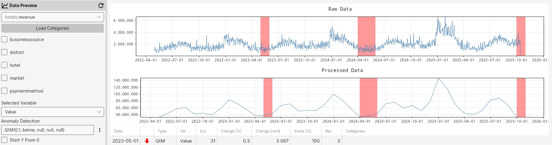
The QtM function detects anomalies in monthly aggregated data by identifying points that fall above or below a defined long-term quantile threshold. It uses the specified quantile and mode ('above' or 'below') to flag extreme deviations within each month’s aggregated values.
Command
QtM(quantile, mode, maxGapAmount, minValue, minCount)
Parameters
quantile- Required. The quantile value for anomaly detection (default value is 0.98)mode- Required. The mode value for anomaly detection - 'above' or 'below' (default value is 'below')maxGapAmount– Maximum allowed proportion of missing data before analysis is skipped (default value is 5%).minValue– Optional minimum value threshold for anomalies (default value is null).minCount– Optional minimum number of points required for detection (default value is null).
Example
QtM(0.98, below, null, null, null);
QtM(0.98, below, 5, null, 10);
QtM();
QtW
The QtW function detects anomalies in weekly aggregated data by identifying points that fall above or below a defined long-term quantile threshold. It uses the specified quantile and mode ('above' or 'below') to flag extreme deviations within each week’s aggregated values.
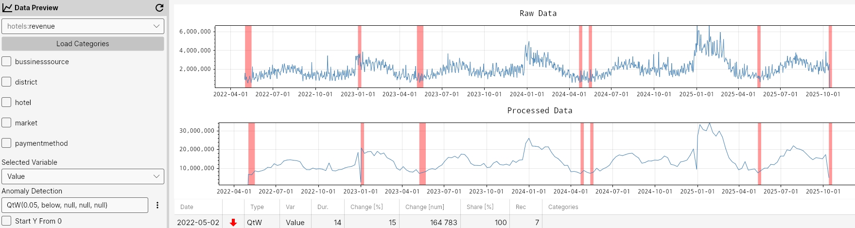
Command
QtW(quantile, mode, maxGapAmount, minValue, minCount)
Parameters
quantile- Required. The quantile value for anomaly detection (default value is 0.98)mode- Required. The mode value for anomaly detection - 'above' or 'below' (default value is 'below')maxGapAmount– Maximum allowed proportion of missing data before analysis is skipped (default value is 5%).minValue– Optional minimum value threshold for anomalies (default value is null).minCount– Optional minimum number of points required for detection (default value is null).
Example
QtW(0.98, below, null, null, null);
QtW(0.98, below, 5, null, 10);
QtW();
Spike
The Spike function detects anomalies by identifying points that exhibit a sudden increase or decrease compared to the rest of the data. It evaluates data in batches of size batchSize and uses a threshold and sensitivity to determine whether a change is significant enough to be considered a spike. Points that sharply deviate beyond these parameters are marked as anomalies.

Command
Spike(threshold, batchSize, sensitivity, maxGapAmount, minValue, minCount)
Parameters
threshold- Required. The threshold value for anomaly detection (default value is 0.35)batchSize- Required. The batch size for anomaly detection (default value is 1024)sensitivity- Required. The sensitivity value for anomaly detection (default value is 99.0)maxGapAmount– Maximum allowed proportion of missing data before analysis is skipped (default value is 5%).minValue– Optional minimum value threshold for anomalies (default value is null).minCount– Optional minimum number of points required for detection (default value is null).
Example
Spike(0.35, 1024, 99.0, null, null, null);
Spike(0.35, 1024, 99.0, 5, 5000, null);
Spike();
WOW
The WoW function detects anomalies by comparing values between consecutive weeks. It flags points where the percentual change exceeds the specified percentualChange in the chosen mode ('above' or 'below'), highlighting sudden increases or decreases from one week to the next.
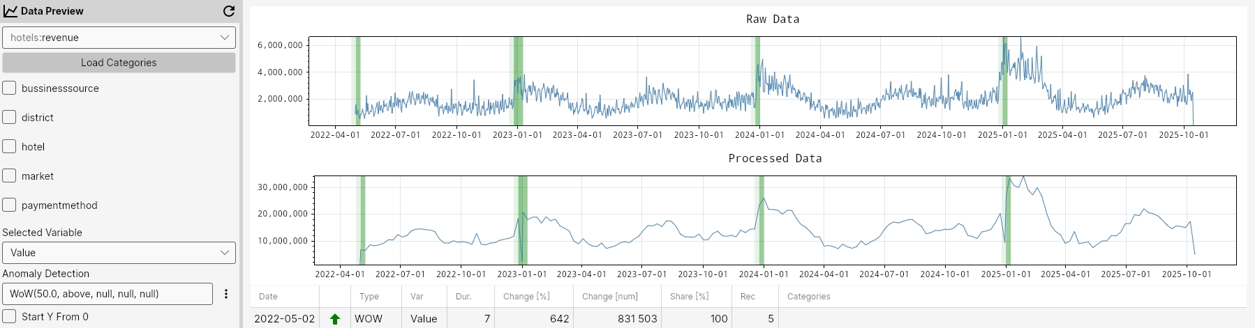
Command
WOW(percentualChange, mode, maxGapAmount, minValue, minCount)
Parameters
percentualChange- Required. The percentual change value for anomaly detection (default value is 50.0)mode- Required. The mode value for anomaly detection - 'above' or 'below' (default value is 'above')maxGapAmount– Maximum allowed proportion of missing data before analysis is skipped (default value is 5%).minValue– Optional minimum value threshold for anomalies (default value is null).minCount– Optional minimum number of points required for detection (default value is null).
Example
WOW(50.0, above, null, null, null);
WOW(50.0, above, 5, null, 10);
WOW();
WPY
The WPY function detects anomalies by comparing values of a given week to the same week in the previous year. It flags points where the percentual change exceeds the specified percentualChange in the chosen mode ('above' or 'below'), highlighting significant year-over-year deviations on a weekly basis.
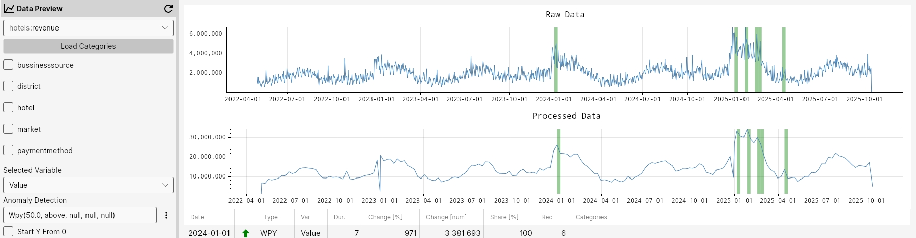
Command
WPY(percentualChange, mode, maxGapAmount, minValue, minCount)
Parameters
percentualChange- Required. The percentual change value for anomaly detection (default value is 50.0)mode- Required. The mode value for anomaly detection - 'above' or 'below' (default value is 'above')maxGapAmount– Maximum allowed proportion of missing data before analysis is skipped (default value is 5%).minValue– Optional minimum value threshold for anomalies (default value is null).minCount– Optional minimum number of points required for detection (default value is null).
Example
WPY(50.0, above, null, null, null);
WPY(50.0, above, 5, null, 10);
WPY();
When the analysis is configured, it can be triggered either via cron or by an external API request. Monitoring analyses is another administrative step that can be performed in AnomalyGuard GUI.