Data Views
Introduction
Data views can be understood as "views on data" that we want to analyze. For AnomalyGuard purposes, we use time series of daily values across selected categories. As an example, we can use a data warehouse of sold products. We have a fact table of sold items organized by products, product groups, countries and regions where they are sold, sales channels, and marketing strategies. Within these categories, there can be tens of thousands of combinations of these dimensions.
| country | region | product group | product | sales channel | marketing strategy | count | sum |
|---|---|---|---|---|---|---|---|
| SK | West | Electronics | Notebook X1 | Online | PPC campaigns | 42 | 58k |
| SK | East | Electronics | Tablet A3 | Retail | Flyers | 27 | 19k |
| CZ | Prague | Home | Mixer M200 | Online | Influencers | 33 | 12k |
| AT | Vienna | Outdoor | Tent Trek 2 | Distributor | Seasonal promo | 18 | 24k |
| HU | Budapest | Food | Bio Snack 50 | Retail | Discount coupons | 56 | 7k |
Normally, a responsible analyst can only control the big numbers - that is, sales across large categories. However, what's important is often hidden in greater detail - in the combination of categories. This is no longer possible to analyze on a daily basis manually. On the contrary, if we have many dimensions with many items, it's simply not possible to analyze everything at once, because there could potentially be millions of these combinations.
Therefore, we create so-called "data views" - views over this data that provide business meaning. As examples, we can create:
- Sales view by country and sales channel
| country | sales channel | count | sum |
|---|---|---|---|
| SK | Online | 42 | 58k |
| SK | Retail | 27 | 19k |
| CZ | Online | 33 | 12k |
| AT | Distributor | 18 | 24k |
| HU | Retail | 56 | 7k |
- Sales view by sales channel and marketing strategy
| sales channel | marketing strategy | count | sum |
|---|---|---|---|
| Online | PPC campaigns | 42 | 58k |
| Retail | Flyers | 27 | 19k |
| Online | Influencers | 33 | 12k |
| Distributor | Seasonal promo | 18 | 24k |
| Retail | Discount coupons | 56 | 7k |
- Sales view by country - product - product group
| country | product | product group | count | sum |
|---|---|---|---|---|
| SK | Notebook X1 | Electronics | 42 | 58k |
| SK | Tablet A3 | Electronics | 27 | 19k |
| CZ | Mixer M200 | Home | 33 | 12k |
| AT | Tent Trek 2 | Outdoor | 18 | 24k |
| HU | Bio Snack 50 | Food | 56 | 7k |
Subsequently, our automated analyses are performed over such data views. Such views are technically "computable" on one hand, and the final results can be combined into one aggregated view at the end.
Note
AnomalyGuard is a powerful tool when your dataset has many categories. It is capable of going through combinations of these datasets, searching for changes and anomalies in them, and aggregating these at the end into an easily readable and actionable form.
AnomalyGuard allows you to create a certain number of such data views that can be analyzed according to your license. With a higher license, the number of Data Views you can analyze also increases.
Input Data
For the purposes of this manual, we use a dataset that describes total revenue and bed occupancy in a hotel chain. Sample data are in the following two tables:
- The first table describes revenue in hotels over time, where we have dimensions assigned to the sum (price) and number of items (count) - business source, hotel, district, market, and payment method.
SELECT * FROM public.hotels_revenue

- The second table describes the development of bed occupancy in hotels (beds), where we have only 2 categories available: hotel and district.
SELECT * FROM public.hotels_beds

Note
AnomalyGuard uses an integer format in YYYYMMDD format for the date dimension. Your input data doesn't have to be directly in this format, because we can request this format in the input data SQL select query.
For analysis, we can load 2 types of numerical values in the input data - value and count. Count is reserved for the number of items and value for the sum or value of the monitored variable (e.g., sales sum, status value of a monitored parameter). In the analysis, we can use either 1 or both parameters.
Data Views Definition
If we want to analyze data, we must create a new Data View in the application. To manage all Data Views, we click on the third button in the side panel - Data View. The application will then display an interface for working with them.

Note
If we want to prepare Data Views, we assume that you have prepared the required connectors to data sources. You can learn more about them in the Connectors section. Like Connectors, Data Views can only be processed by a user with Admin rights.
Initially, the data views window is empty. If we want to add a new Data View, we click on the Plus button (+) in the side panel. Subsequently, a dialog for Data View definition will appear in the main window.
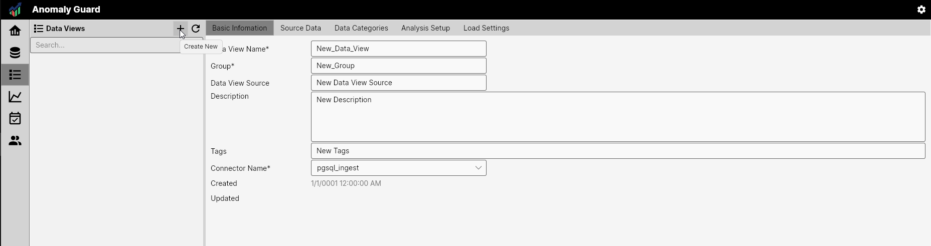
In this window, we define the entire Data View - its metadata, SQL query formulation, dimensions, change and anomaly analysis, and its orchestration. The definition is divided into 5 sections, each focused on a specific part:
- Basic Information (basic information and metadata about Data View)
- Source Data (definition of source data acquisition)
- Data Categories (category setup - data dimensionality)
- Analysis Setup (change and anomaly analysis settings)
- Load Settings (regular load parameter setup)
Basic Information
In the first tab, we define basic information about the Data View. We must define Data View Name, Group, and Connector Name as mandatory fields. Others form auxiliary metadata that is useful for describing the Data View. These parameters gain importance when a larger number of people use this tool or its results, or when we have a large number of analyzed Data Views.
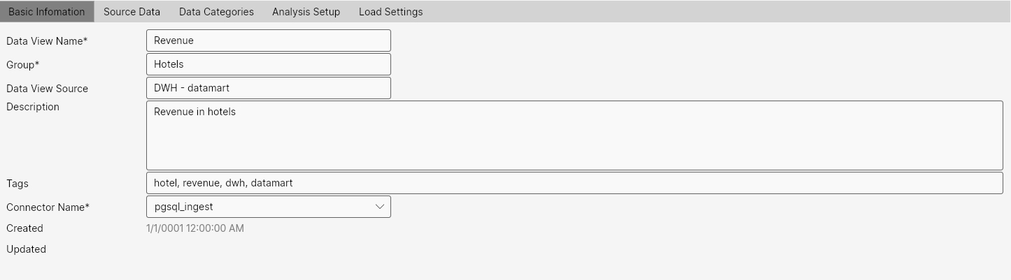
-
Data View Name: Required. Name of the new Data View. The name defines the view and should be understandable. As examples for our case, we can use names like Beds, Beds_Occupancy, Revenue_In_Counties, Revenue_Per_Product_Group. Naming is optional according to customer needs.
-
Group: Required. Individual Data Views should be divided into Groups. The design of these groups is up to the customer and can define, for example, business domains (e.g., HR, Sales, Marketing, ...), source data domains (e.g., DWH, CRM, IT, ...), or other types of groups. Under these groups, we should find similar Data Views.
-
Data View Source: Optional information about the source of data that is analyzed by this data view (e.g., DWH, CRM, ...).
-
Description: Optional. Longer description of the Data View. This parameter should sufficiently define the Data View so that the end user knows what data and how it is analyzed.
-
Tags: Optional. Tags defining the Data View. Used, for example, when searching and filtering data views in the application.
-
Connector Name: Required. Name of the connector through which data will be downloaded from the source system. Individual connectors are defined in the Connectors section.
-
Created: DateTime. Information that defines when the Data View was created.
-
Updated: DateTime. Information that defines when the Data View was last updated.
Once we have defined all this data, we can proceed to the source data setup.
Source Data
Source data is defined in the application on the second tab - Source Data. In this tab, we define 2 types of queries. The first - Load Query is mandatory and will be used for regular loading. This means it should provide current data, for example, for incremental load D-1. In case there is relatively little data, we can also use a simpler full load, where the query returns a dataset for the entire analyzed period. Incremental loads are suitable when we would have to load tens and millions of rows daily with a full load.
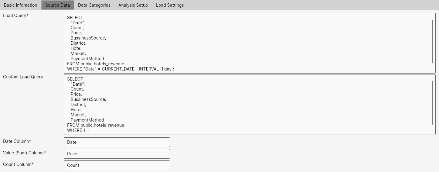
The following section shows a sample example for Load Query:
SELECT
    "Date",
    count,
    price,
    "BussinessSource",
    "District",
    "Hotel",
    "Market",
    "PaymentMethod"
FROM public.hotels_revenue
WHERE "Date" = CURRENT_DATE - INTERVAL '1 day';
The second - Custom Load Query serves to define "custom load". This serves, for example, for initial full load or for a custom query that provides corrected data for a longer time period. After saving, we can run the load through this query manually in the GUI. The procedure will be explained in a later chapter.
Using the last three text boxes - Date Column, Value (Sum) Column, and Count Column, we define the column names in the output from queries that contain values for Date, Value, and Count. These parameters are mandatory.
Warning
1) The date input to the application must be in integer format YYYYMMDD. If you have a date component in the source DB in format like DateTime, use a modification in the select similar to the following example:
CAST(to_char("Date", 'YYYYMMDD') AS int) AS date_int
2) Values for count and value must be in some numeric format. Other categorical variables should be in text form.
3) In both query definitions, we recommend not using the style:
SELECT * FROM TableA
Always use precise column identification. This will help you avoid several problems in the future.
4) If in both queries you are pulling data for a selected day, always provide all data for that date. Incremental load works by extracting a list of dates for which we have data from new data, and values for these dates are deleted and then new data is loaded.
5) The output query must (in the current version) contain both values. If we are analyzing a dataset that has only Value or Sum value, we define the unused value in the query as a constant:
SELECT 1 as 'Count' FROM ....
6) The output column names in the SELECT must match the names used in Data Categories in the Name column.
Data Categories
When we have defined the source query and know which columns contain Date, Count, and Value values, we can continue with the setup of dimensions - categories. On the Data Categories tab, we define individual categories.
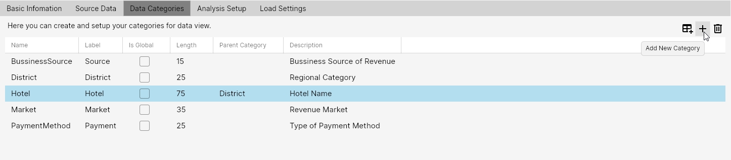
- Name: Category name from SQL Select. Using this parameter, we find data in the query output.
- Label: Category name in the application. If we require different naming for the category in the query from the source system and different in the application output (e.g., for simplification and improved readability), we define its modified name.
- Is Global: Variable planned for future development. Will be used for overall analyses over globally used dimensions (e.g., region). Currently not used.
-
Length: Maximum number of characters that can be used within the variable in the result table. This number must be higher than MaxLength for the category. To determine this length, we use something like:
SELECT MAX(LENGTH(columnA)) AS max_data_length FROM tableA; -
Parent Category: If we use hierarchical categories (e.g., country - region - city or product line - product group - product), we define the parent category for the current category. Used to reduce the number of combined dimensions when analyzing data so that, for example, data for cities in regions where they are not located is not searched. In one Data View, we can have multiple hierarchical dimensions - e.g., region and product.
- Description: Optional. This box can be used to describe the category.
When we have defined these data categories, AnomalyGuard knows in which dimensions and their combinations it can analyze and search the input data.
Analysis Setup
In this step, we have defined source data and dimensions in which we will operate. On the next tab - Analysis Setup, we will define the analyses that will be processed on the data.
In the first listbox Analyzed Variables, we define variables that we want to analyze. We can select one or more variables - Count, Value, and Avg. The first two we define directly in the data. The last variable Avg is calculated from the data (Avg = Value / Count).

Another parameter is Fill Gap Method. In input data, we can have gaps - dates for category combinations when we have no data. Using this parameter, we determine how AnomalyGuard should perceive this missing data. If it's about sales sums, for example, it's clear that it's either a data outage or we really have no values for the given time and thus sales for that date are zero. But if it's about status values, such as air temperature, missing data means rather an outage in values and not a zero value. Using this parameter, we define how the application should perceive it - whether it should fill in a zero value (Zero), interpolate data between the last and next known (Linear Interpolation), or use the last known (Previous).
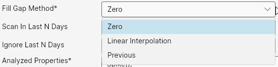
Another configurable parameter is Scan In Last N Days. Using this parameter, we can limit how many last N days will go into analysis. It may happen that we have, for example, 10 years of data. However, the COVID period brought large anomalies to the data, which we no longer want to have included in the data today. Or due to the size and complexity of the analyzed dataset, we want to increase the speed of analysis. In these cases, we can, for example, limit the length of data series to the last 3 years. If the value is set to 0, all available data will be used for analyses.
Using another parameter Ignore Last N Days, we can conversely adjust the so-called "data freshness". This can help in case we have a dataset that contains so-called "Late Arriving Facts" - meaning that part of the data arrives, for example, to the data warehouse later. Then it may happen that the last days will show anomalous values despite the fact that the data is temporarily incomplete. To avoid this, we can define this integer value. Subsequently, the last N days will always be ignored in analyses. If the value is equal to zero, all data will be used.
Finally, we have the editor for the Analyzed Properties parameter. In this text box, we define all detection algorithms that we want to use on the Data View. Individual algorithms are defined as simple functions separated by semicolons. Using the last Help combobox, we can display basic documentation for individual detectors.
Note
Setting up detection algorithms is a more demanding and complex task and therefore it has a dedicated chapter in the Analysis Setup section.
Load Settings
On the last tab - Load Settings, we define load parameters - how we will start the load and what type of load it will be. Using the first parameter Load Mode, we define whether it will be a full load or incremental load. According to this, new data is either merged (Incremental) or completely overwritten (Full).
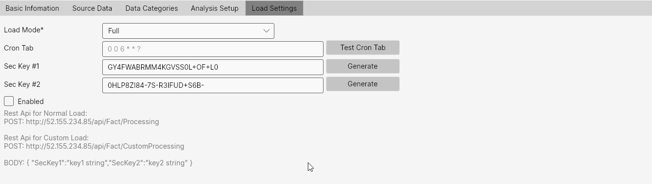
Using the Cron Tab parameter, we can define the timing for starting regular loads. Through cron, we can define when the load will be executed.
Cron definition
We define Cron using six fields:
| sec | min | hour | day | month | day-of-week |
|---|---|---|---|---|---|
| * | * | * | * | * | * |
| 0–59 | 0–59 | 0–23 | 1–31 | 1–12 | 0–6 |
Basic rules for fields:
- Numbers in the range of each field.
-
- = any value.
- Interval */n = every n units.
- List a,b,c = specific values.
- Range a-b = from a to b.
- day-of-week: 0 = Sunday, 6 = Saturday (most libraries).
- Conflict "day" vs "day-of-week" usually works as OR, not AND.
Cron examples:
- Every day at 03:00:
0 0 3 * * * - Every Saturday at 06:00:
0 0 6 * * 6 - First day of each month at 01:00:
0 0 1 1 * *
Cron start: - An active cron will start a new daily load only if there is no other job currently in progress (e.g. a previous daily load, a custom load, or a custom analysis).
If the Cron Tab value is empty, the analysis will not be performed automatically at the defined time. In that case, we can run the data load and analysis either manually through this GUI (see last section) or we can run it from an external system via POST API request.
This external triggering approach is suitable when we need to first consolidate data and only then run processing in AnomalyGuard - for example, after daily data load to the data warehouse or data product. This way we can ensure that the analysis will be performed on processed and complete data.
Externally triggered data load is done via POST API request to the URL that is displayed on this tab. The first URL is prepared for daily load and the second for custom load. We don't need to authenticate the request for execution. However, in the POST request, we need to send 2 security keys. These must be unique for all Data Views and we define them through text boxes Sec Key #1 and Sec Key #2.
The last configurable parameter is the Enabled checkbox. This checkbox activates or deactivates data processing. If a trigger is activated or processing is started via API, processing will run only if the Enabled parameter is TRUE.
Data Views Management
In the main window you define the parameters for each Data View. After adding a Data View it appears in the side panel where Data Views are managed. From the side panel you can add a Data View, edit it using the visible buttons, or manage it via the context menu that appears under the three-dots button.
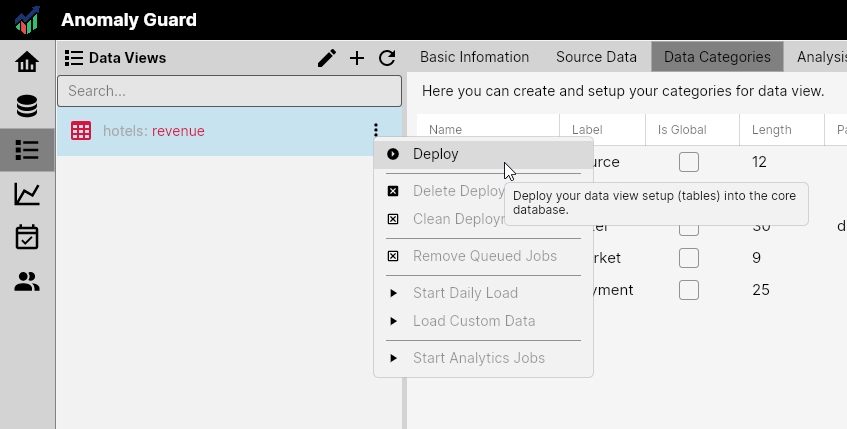
When a new Data View is added it is initially shown in red. This means the Data View definition is ready but the required database objects (tables and indexes) have not yet been generated.
To start working with a Data View, click Deploy in the side menu. AnomalyGuard will then generate all required database objects and display a success notification in a message box.

Deployment Status
If a Data View is not in state Deployed = TRUE, you can edit all settings and context-menu functionality is limited to the Deploy command.
After deployment you cannot edit parameters under the Data Categories tab because they are directly tied to generated DB objects. If you need to change categories later, you must remove the deployment via the context menu option Delete Deployment and then reload and re-run the analysis.
Conversely, after deployment the context menu functions for managing Data View jobs are activated — manual start of daily load and analysis, custom data loads, or starting analysis on the current dataset.
After a successful deployment the Data View color changes from red to black. Individual context-menu functions become active and two additional commands become available:
- Delete Deployment (remove all Data View objects from the database — helper tables and indexes)
- Clean Deployment (delete contents of Data View DB objects — cleanup)
Other context-menu items remain unavailable until you enable the Data View. To do that, set Enabled = TRUE on the Load Settings properties tab and save.
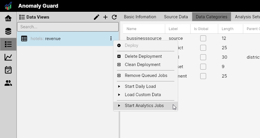
The Data View color will then change from black to green.
Data View Enabled status
When a Data View is set to Enabled it becomes active. If a Cron is defined for data loads, it will start running. Analyses can also be triggered via the REST API. The Data View is also activated across related areas — Data Preview, User Access Administration, and Anomaly Filters.
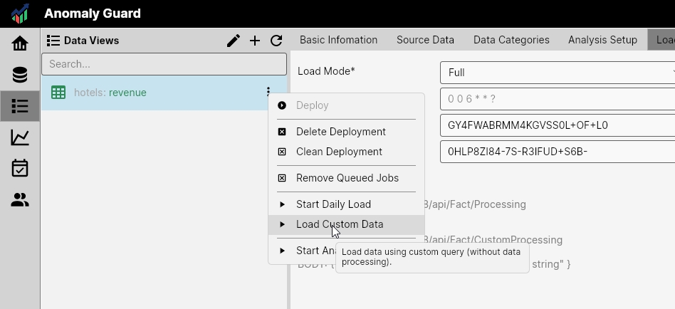
You can then run the following context-menu functions for the Data View:
- Remove Queued Jobs — removes queued jobs for data loads and analysis jobs. Use this if you detect an issue in the analysis (e.g., inaccessible source data or an incorrectly defined analysis).
- Start Daily Load — starts the daily load (runs the configured Load Query) and then executes the defined analytical jobs. Use to manually run the complete daily job.
- Load Custom Data — runs the Custom Load Query to manually load customized data (e.g., initial or corrective loads). This command does not automatically start analytical jobs.
- Start Analytics Jobs — starts analytical jobs without importing new data (runs on currently loaded data). Use after a custom data load or after updating detection algorithms or Data View settings.
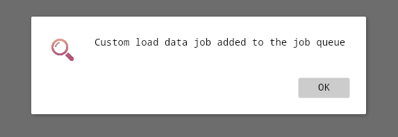
After a process starts successfully, a message box notifies the user.
Editing Data Views and process management
Only users with Administrator rights in the application can modify settings and start processes.